 Version 4.41
has a few improvements such as dart launches,
easier editing and it now has optional launch
tube (hollow with a specified empty length),
T-nozzle, parachute (with deployment at
apogee or timed from the launch) and air
impulse. Version 4.41
has a few improvements such as dart launches,
easier editing and it now has optional launch
tube (hollow with a specified empty length),
T-nozzle, parachute (with deployment at
apogee or timed from the launch) and air
impulse.In addition to
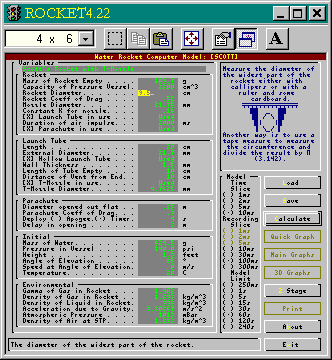
this, there is context sensitive help (shown
on the left with a tip on how to measure the
diameter 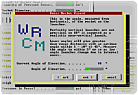 of your rocket) and tips on
reasonable values such as coefficient of drag and
so on. If you are using the Novice
option, there is even a wizard that allows the
meaningful input of data - especially useful for
young students. of your rocket) and tips on
reasonable values such as coefficient of drag and
so on. If you are using the Novice
option, there is even a wizard that allows the
meaningful input of data - especially useful for
young students.
Further, the model is faster as
it does not write the data file to disc but
stores information taken at regular intervals in
memory. This recording time slice can be altered
as can the runaway-limit on the model - making a
small recording-time-slice and short model-run
allows the study of the first few seconds of the
flight. You can now print out a full report on
the rocket from input parameters, model settings
and results
It is shown here, running in a
DOS box under Windows 95 - choose a font size
that suites you or run it full screen by pressing
[Alt][Enter]. (It is shown here with a 4 x 6
font to keep the image small. I would recommend
at least 6 x 8 although 8 x 12 is preferable.)
|
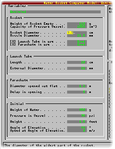 In addition to
the 'expert' version, you can opt to use a
simplified 'novice' version to get to know the
basics of the model without having too many
parameters to change. Once you have familiarised
yourself with it, go onto the expert version
where you will be able to change more variables. In addition to
the 'expert' version, you can opt to use a
simplified 'novice' version to get to know the
basics of the model without having too many
parameters to change. Once you have familiarised
yourself with it, go onto the expert version
where you will be able to change more variables. At the very beginning of the model, you
are offered a choice of units for height in feet
or metres and pressure in psi or Bar. The
files that are saved are all in SI so you will be
able to exchange these regardless of units
selected.
|
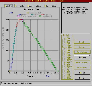 Once the
calculation has been made, you have the option of
quick graphs, including statistics, and graphs of
height, velocity and acceleration against time. Once the
calculation has been made, you have the option of
quick graphs, including statistics, and graphs of
height, velocity and acceleration against time.The quick graphs all use the standard
text display (shown on the left) and
should work on any computer therefore users will
not find themselves without any graphs
should their machine not have the correct
display.
The graphs of Height, Velocity
and Accelerations against time all use colours to
denote periods of launch tube, water
thrust, air impulse, coasting, chute
opening and full deployment.
|
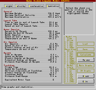 In addition, a
table of statistics can be displayed showing most
of the numbers that rocketeers should be
interested in when testing in this way (it is
impossible to please everyone though). In addition, a
table of statistics can be displayed showing most
of the numbers that rocketeers should be
interested in when testing in this way (it is
impossible to please everyone though). |
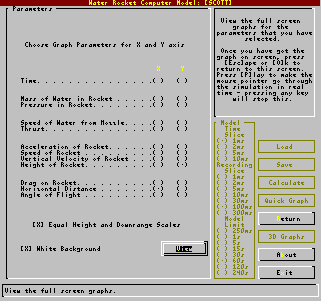 Further to the quick graphs
are the graphs using the VGA display (keeping
it down to just VGA should include most people). Further to the quick graphs
are the graphs using the VGA display (keeping
it down to just VGA should include most people).On
the screen shot on the left, you can see that the
X axis does not have to represent time but can,
instead, represent any of the variables so,
should you be inclined so, you can have a graph
of Height against Drag or Velocity against
Acceleration.
|
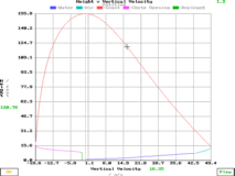 This is a plot of height against
velocity - such a graph giving the optimum time
and details for calculating a second stage
deployment. This is a plot of height against
velocity - such a graph giving the optimum time
and details for calculating a second stage
deployment.You can
select a black or a white coloured background -
white resulting in less ink use when printing out
from the screen.
|
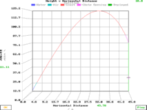 If your rocket travels a significant
distance downrange, you can choose to see it with
the horizontal and vertical scales the same.
Also, you can click on Play to
get the computer to move the cursor along the
line in real time. If your rocket travels a significant
distance downrange, you can choose to see it with
the horizontal and vertical scales the same.
Also, you can click on Play to
get the computer to move the cursor along the
line in real time. |
 The program
includes a 3 dimensional graph plot which
calculates an output result (such as maximum
height, velocity, acceleration, time to apogee or
flight time) against two input variables
such as mass of empty rocket and diameter of
nozzle. If you are using a launch tube, you can
vary the length of this as well and if it is a
hollow tube, the length of the empty part of the
tube may be specified as remaining the same
length (such as if you were using a T-nozzle
and had small holes in the launch tube), the
same proportion (such as if you filled the
rocket using the launch tube and you only managed
to blow a certain proportion of the water out
when pressurising the rocket) or a fixed
filled part (such as if you had a particular
launcher that you could put various lengths of
launch tube onto). The program
includes a 3 dimensional graph plot which
calculates an output result (such as maximum
height, velocity, acceleration, time to apogee or
flight time) against two input variables
such as mass of empty rocket and diameter of
nozzle. If you are using a launch tube, you can
vary the length of this as well and if it is a
hollow tube, the length of the empty part of the
tube may be specified as remaining the same
length (such as if you were using a T-nozzle
and had small holes in the launch tube), the
same proportion (such as if you filled the
rocket using the launch tube and you only managed
to blow a certain proportion of the water out
when pressurising the rocket) or a fixed
filled part (such as if you had a particular
launcher that you could put various lengths of
launch tube onto). |
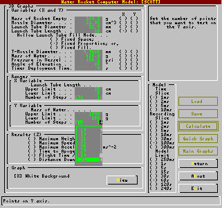
 The number of points along each axis may
be specified (between 1 and 31 - 1 if you are
interested only in optimising against one input
parameter) and if you are only looking at
something that happens early on in the flight
such as maximum velocity, you can specify a short
model run time to make filling the points
quicker. Another trick to speeding up the process
is to select a longer model calculation interval
- selecting 10ms will make the model 10 times
faster with granularity showing only in time to
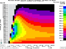
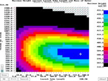
apogee. The graph on the left shows Maximum
Height (z axis) plotted against Mass of
Water (y axis) and T-Nozzle Diameter (x
axis). This shows the best fill and T-Nozzle
diameter. The number of points along each axis may
be specified (between 1 and 31 - 1 if you are
interested only in optimising against one input
parameter) and if you are only looking at
something that happens early on in the flight
such as maximum velocity, you can specify a short
model run time to make filling the points
quicker. Another trick to speeding up the process
is to select a longer model calculation interval
- selecting 10ms will make the model 10 times
faster with granularity showing only in time to
apogee. The graph on the left shows Maximum
Height (z axis) plotted against Mass of
Water (y axis) and T-Nozzle Diameter (x
axis). This shows the best fill and T-Nozzle
diameter. The
distribution of the colours on the graph may be
changed by clicking the mouse on the colour scale
on the right - moving this up will make the upper
colours represent a narrower range and so on.
Doing this allows you to see how well you can
optimise your flight.
|
 When using a
hollow launch tube, the length of empty tube may
be specified on the main model sheet in the main
values above. On the 3 dimensional graph values
form, you can specify whether you want the model
to consider the hollow part of the launch tube in
terms of a fixed measurement of space (10cm
empty of a variable length tube - specified on
the main variables form as a 20cm tube), When using a
hollow launch tube, the length of empty tube may
be specified on the main model sheet in the main
values above. On the 3 dimensional graph values
form, you can specify whether you want the model
to consider the hollow part of the launch tube in
terms of a fixed measurement of space (10cm
empty of a variable length tube - specified on
the main variables form as a 20cm tube), |
|
Fixed space used for tubes in
rockets that are filled slowly - ie, only have a
certain volume of air in the water |
 a proportional
measurement of space (50% empty) or, a proportional
measurement of space (50% empty) or, |
|
Proportional spaced tubes used
for tubes in rockets that are pressurised quickly
so that a fixed proportion of the tube is air
with the rest water. |
 a fixed
measurement of filled launch tube (10cm of
the tube is not empty ie 20cm - 10cm). Each
of these three senarios have a different role to
play and the computer model can match these. a fixed
measurement of filled launch tube (10cm of
the tube is not empty ie 20cm - 10cm). Each
of these three senarios have a different role to
play and the computer model can match these. |
|
Fixed fill tubes used for tubes
with a fixed portion filled by, say, a T-nozzle
support or an adaptor - something that occupies
the same volume regardless of the length of the
tube, or tubes that are always dry - ie,
compressed air only. |
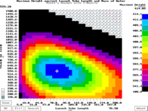
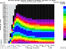 In addition to this, you may elect to
view the graph row by row or column by column so
as to produce a graph that shows, say, the
optimum mass of water for each given T-nozzle
diameter as in the graph on the left. In addition to this, you may elect to
view the graph row by row or column by column so
as to produce a graph that shows, say, the
optimum mass of water for each given T-nozzle
diameter as in the graph on the left.Selecting Fill whilst the graph is split
in this way will fill just one row or column.
|
 Version 4.41 includes an automatic Version 4.41 includes an automatic  search that
will locate the maximum in the current graph for
you without having to calculate all of the points
- only needing to calculate around 5% of points
on a 31 x 31 plot and doing that many times
quicker than by hand. search that
will locate the maximum in the current graph for
you without having to calculate all of the points
- only needing to calculate around 5% of points
on a 31 x 31 plot and doing that many times
quicker than by hand. It
starts where you click the mouse and then finds a
direction of increasing output parameter and
follows it until it finds that it starts to
decrease and then changes direction again - 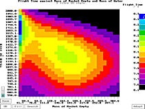 keeping on doing this until it has
located a maximum. It is able to do this many
times quicker than doing it manually because it
looks at the numbers rather than the colours. keeping on doing this until it has
located a maximum. It is able to do this many
times quicker than doing it manually because it
looks at the numbers rather than the colours.
Plots of Maximum height,
velocity, acceleration and so on may be viewed
simply by pressing keys to switch between plots
without recalculating all of the points.
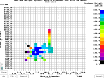
There are limitations to
automatic searches in that where there is more
than one maximum, the search may find the wrong
one. The graph on the right is of rocket weight
and water weight with flight time as the output
parameter. For a really lightweight rocket, the
thrust pushes the rocket up into the air which
then floats to earth (not having much weight to
pull it through the viscous air :-).
|
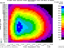 Version 4.41 allows you to look at chute
deployment times showing some interesting results
as in the screen shot on the left which is of
flight time plotted against deployment time (Y
axis) and mass of water (X axis).
This is with a 4 metre chute opening delay (the
distance that it takes for the chute to open
fully from Version 4.41 allows you to look at chute
deployment times showing some interesting results
as in the screen shot on the left which is of
flight time plotted against deployment time (Y
axis) and mass of water (X axis).
This is with a 4 metre chute opening delay (the
distance that it takes for the chute to open
fully from 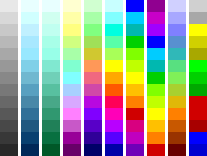 the point of release). the point of release).Pressing [A]dopt and then clicking on a
point will put the x and y values back into the
input parameters form and the 3D form and allow
you to optimise two other variables thus speeding
up the optimisation process even more.
Pressing [SpaceBar] will change
the colour set to one of those on the right.
|
| Version 4.41 introduces a 2 stage
optimisation which you can use to make sustainer
and booster files interact for maximum height or
range. This includes crushing sleeve and
expanding tube release mechanisms. Files can be
optimised or simply ran as a two stage rocket. |